Top Basic Excel Interview Questions in 2025 for Freshers
Table Content
Introduction
Welcome to our Excel Mastery Course! Whether you’re looking to enhance your data analysis skills or streamline your workflow, this course is designed to equip you with the knowledge and tools to excel in Excel. From basic functions to advanced techniques, join us as we navigate through practical lessons and hands-on exercises to help you become a proficient Excel user. Let’s dive in and unlock the full potential of Excel together!
1. What is Microsoft Excel?
Microsoft Excel is an electronic spreadsheet application that enables users to store, organize, calculate, and manipulate data with formulas using a spreadsheet system broken up by rows and columns. It also provides the flexibility to use an external database to do analysis, make reports, etc. thus saving lots of time.

2. How Many Excel Data Formats Are Available? Name Them.
Six. They include:
- Excel workbook: .xlsx
- Excel macro-enabled workbook: .xlsm
- Excel binary workbook: .xlsb
- Template: .xltx
- Template (code): .xltm
- XML data: .xml

3. What’s in Excel for a Cell Address?
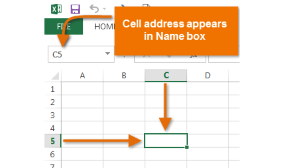
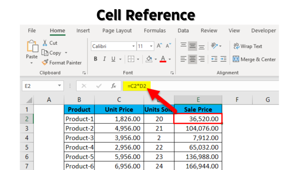
A cell address (or cell reference) is made up of the row letter and column number a cell is located in. The cell in row D, column 7 has the cell address of D7. Cell addresses are used in formulas when giving spreadsheet instructions but are also used in general communication to specify cells.
4. What Is Absolute Cell Reference in Excel?
Absolute cell referencing is the exact opposite of relative cell referencing. By marking the row number and column letter with a $ symbol, you can make a cell reference fixed (or “absolute”).
This means that when you copy and paste it to another cell or use AutoFill, the cell references will not change. The formula =SUM(A4:A8) will stay as =SUM(A4:A8) no matter where you put it.
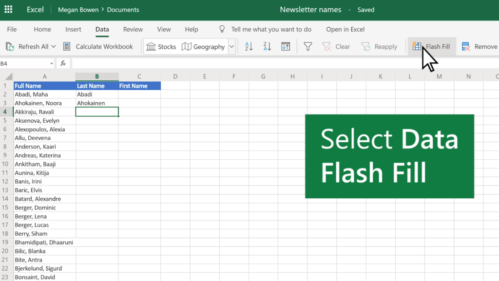
5. What is the purpose of Flash Fill, and how do you activate it?
Flash Fill is an Excel feature that can be used to quickly fill cells with data based on user behaviors. Flash Fill is often turned on by default, so to use it you can begin typing. If Excel identifies a pattern, the program will suggest data for the cell. You can press enter to accept suggested data in Flash Fill. If Flash Fill is turned off, you can activate it by selecting Tools > Options > Advanced > Editing Options and clicking the checkbox that says “Automatically Flash Fill.
6. What Are the Downsides of Microsoft Excel?
Microsoft Excel is a proprietary, paid solution, so not everyone uses it. Some prefer free solutions like Google Sheets. Microsoft Excel is primarily used as a spreadsheet to collect data and perform minor analysis functions, so it might not be ideal for complex database tasks.

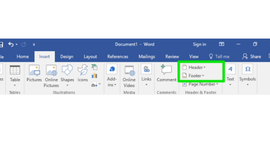
7. What Is a Header or a Footer?
Like Microsoft Word, a header and footer in Excel are displayed at the top and bottom of each page in a worksheet. You can customize these headers and footers to include the date, time, sheet name, and more.
8. What Are the Major Competitors of Excel?
Google Sheets, Zoho Sheets, and LibreOffice are common spreadsheet applications and alternatives to Excel. For analytics purposes, MATLAB and PowerBI are ideal, and you can even create an SQL database like MySQL to crunch larger volumes of more complex data.
9. Explain a few useful functions in Excel.
Following are the functions available in Excel for manipulating the data:
- Math and Financial Functions – SQRT, DEGREE, RAND(), GCD
- Logical Functions – IF, AND, FALSE, TRUE
- Date and Time functions – NOW(), DATEVALUE(), WEEKDAY(NOW())
- Index Match – VLOOKUP and INDEX MATCH
- Pivot tables
10. Is it possible to create a Pivot Table using multiple data sources?
Yes, you can create a pivot table from multiple worksheets. For this, there must be a common row in both the tables. This will act as the Primary key for the first table and the Foreign key for the second table. Create a relationship between the tables and then build the pivot table.
11. What about filtering?
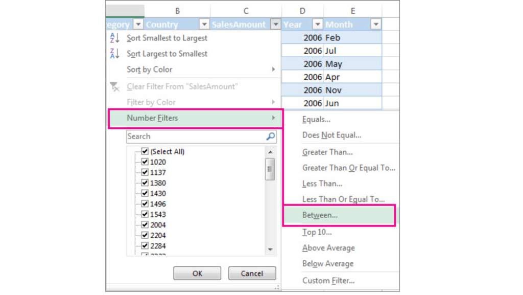
Filtering data in Excel allows you to display only the rows that meet certain criteria. To apply a filter, click on the Data tab, then select Filter – dropdown arrows will be added to each column header. Use these dropdown menus to filter the data.
12. What is the Vlookup function in Excel?
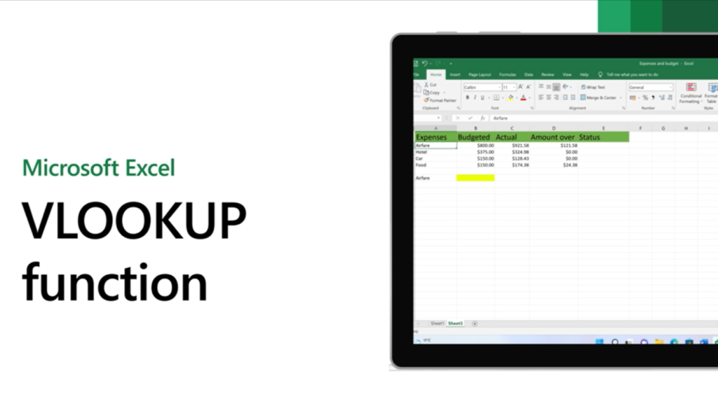
VLOOKUP function searches vertically in columns of data. It returns a value from a different column in the same row.
Formula –
=VLOOKUP(lookup_value, table_array, col_index_num, [range_lookup])
13. How do you format the data in Excel?
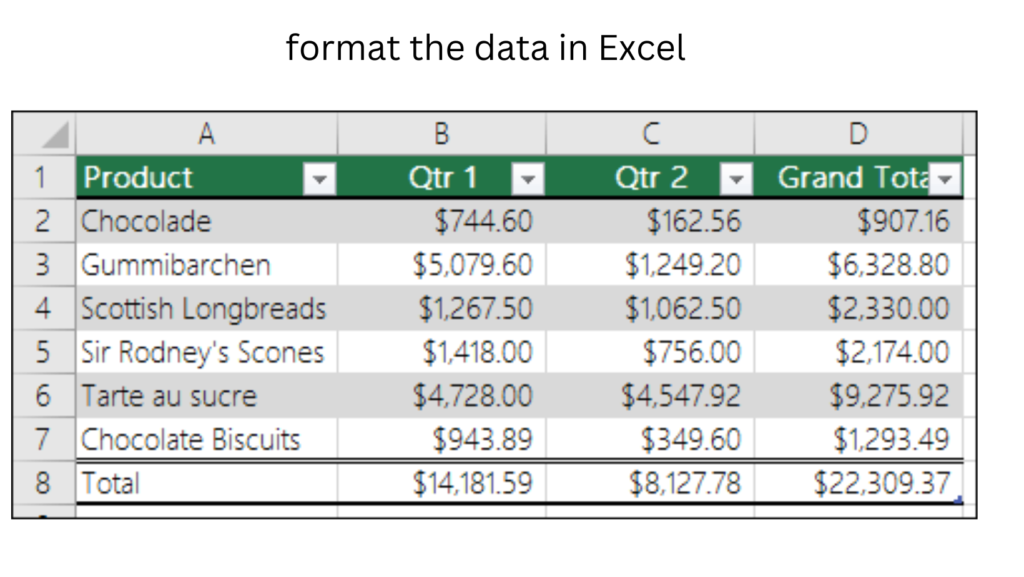
In Excel, data formatting is adjusted using the options in the Home tab, where you can change the font type, size, color, cell borders, and background color. For numerical data, right-click a cell or range, select Format Cells, and choose from categories like Number, Currency, Date, or Custom to format the data as desired. Conditional Formatting, also found in the Home tab, allows you to automatically format cells based on their values, such as highlighting cells that contain numbers above a certain
threshold.
14. What is the shortcut to applying a formula to an entire column in Excel?
You can double-click on the bottom right corner of the cell to apply a formula to an entire column in Excel.
OR
If the cell already has the formula, you can apply it as follows:
Select the cell containing the formula and press CTRL+SHIFT+DOWN to select the rest of the column
Press CTRL+D
Use CTRL+UP to return up
OR
If the formula is in the first cell of a column –
Select the entire column by clicking the column header or any cell in the column
Press CTRL+SPACE
Fill the consecutive cells using CTRL+D
15. How do you sort the data?
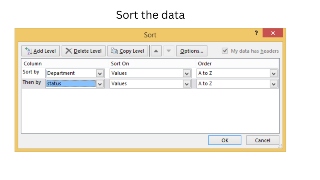
First, select the range of cells you want to sort to sort data in Excel. Click on the “Data” tab in the ribbon at the top of Excel. Click on the ‘Sort’ button to open the Sort dialog box. Then, choose “Sort A to Z” for ascending order or “Sort Z to A” for descending order if sorting alphabetically. You can also apply custom sorting criteria from the Sort dialog box. Remember to check the “My data has headers” option if your data includes headers to ensure they are not included in the sorting process.
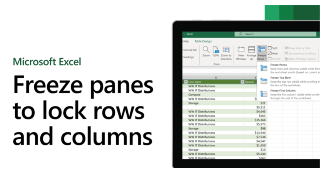
16. How can you freeze panes in Excel?
To freeze panes in Excel, ensure that certain rows or columns remain visible as you scroll through your spreadsheet. First place your cursor in the cell immediately to the right of the column and below the row you want to freeze. Go to the ‘View’ tab on the Ribbon, and in the ‘Window’ group, click on ‘Freeze Panes’. From the drop-down menu, select ‘Freeze Panes’ to freeze the rows above and columns to the left of your selected cell. This feature is particularly useful for keeping headers visible while scrolling through large datasets.
17. How do you create a pivot table?
To create a Pivot Table in Excel, first select the data range you want to analyze. Next, go to the “Insert” tab on the ribbon and click on “PivotTable.” In the dialog box that appears, choose where you want the Pivot Table to be placed (new worksheet or existing worksheet). After clicking “OK,” the PivotTable Field List pane will appear, where you can drag fields to the different areas (Rows, Columns, Values, and Filters) to organize your data.

18. How do you protect a Workbook?
To protect an entire workbook in Excel, navigate to Tools > Protection > Protect Workbook. Enter a password in the dialog box that appears, and then re-enter it when prompted for confirmation. This will encrypt the workbook, requiring the password to open it in the future
19. How do you create a drop-down list from a data validation?
To create a drop-down list in Excel using data validation, first select the cell or cells where you want the drop-down list to appear. Then, go to the “Data” tab on the ribbon and click on “Validation”. In the Data Validation dialog box, under the “Settings” tab, select “List” from the “Allow:” dropdown menu.
In the “Source:” box, either type in the list items separated by commas, or click the up arrow button to select a range of cells containing the items you want in your list. Ensure that the “In-cell dropdown” box is checked. Click “OK” to apply the data validation and create your drop-down list.

20 . How Can You Import Data From Another Workbook?
Microsoft Excel makes it easy to import data from another workbook. You can create an external reference between workbooks by typing the source workbook name and the sheet you are pulling data from, as shown in the command below.
data from: =[SourceWorkbook.xlsx]Sheet1!$A$1 |
Note that if the file is moved, the sheet is renamed, or the data is shifted, the data that is pulled will be incorrect.
For Excel training, Anubhav offers:
Enrolling in Anubhav for Excel training provides several compelling advantages:
- Expert Instructors: Learn from experienced Excel professionals who provide comprehensive guidance and practical insights, ensuring a deep understanding of Excel features and functions.
- Comprehensive Curriculum: The Excel training curriculum covers all essential topics, from basic spreadsheet operations to advanced data analysis techniques and automation using macros and VBA (Visual Basic for Applications).
- Hands-on Learning: Emphasis is placed on hands-on experience with practical exercises, projects, and real-world examples. This interactive approach helps reinforce understanding and develop practical Excel skills.
- Industry Connections: Students have the opportunity to network with industry professionals and experts through guest lectures, workshops, and networking events. This exposure provides valuable insights into Excel usage across various industries and potential career opportunities.
- Flexibility and Convenience: Anubhav offers flexible training options, including online and in-person classes. Students can choose the format that best fits their schedule and preferences, ensuring a convenient learning experience.
- Affordable Pricing: Despite offering top-quality training, Anubhav’s Excel programs are priced competitively. Students receive excellent value for their investment, gaining valuable skills that can enhance their productivity and career prospects.
In summary, enrolling in Anubhav for Excel training provides a comprehensive and flexible learning experience led by expert instructors, making it an excellent choice for mastering Excel skills.
